import numpy as np
import pandas as pd

class cdc_risk:
    def __init__(self, base_risk = 0.00003):
        self.base_risk = base_risk

    def predict(self, x):
        rratio = np.array([7900] * x.shape[0])
        rratio[x.Age < 84.5] = 2800
        rratio[x.Age < 74.5] = 1100
        rratio[x.Age < 64.5] = 400
        rratio[x.Age < 49.5] = 130
        rratio[x.Age < 39.5] = 45
        rratio[x.Age < 29.5] = 15
        rratio[x.Age < 17.5] = 1
        rratio[x.Age < 4.5] = 2
        return rratio * self.base_risk

model_cdc = cdc_risk()
steve = pd.DataFrame({"Age": [25], "Diabetes": ["Yes"]})
model_cdc.predict(steve)
## array([0.00045])Step 0. Hello model!

Predictive models have been used throughout entire human history. Priests in ancient Egypt could predict when the Nile would flood or a solar eclipse would come. Developments in statistics, increasing availability of datasets, and increasing computing power allow predictive models to be built faster and deployed in a rapidly growing number of applications.
Today, predictive models are used everywhere. Planning of the supply chain for a large corporation, recommending lunch or a movie for the evening, or predicting traffic jams in a city. Newspapers are full of exciting applications. But how are such models developed?
In this book we will go through the full cycle of training and testing of predictive models. We’ll load the data, explore it, build some models, and move on to the main part of this book - detailed model analysis using eXplainable Artificial Intelligence (XAI) techniques. The core intuition behind these methods is presented in consecutive sections. If you would like to learn more about discussed methods, a detailed introduction to them can be found in the book Explanatory Model Analysis (Biecek and Burzykowski 2021) (available in paperback and online).
Biecek, Przemyslaw, and Tomasz Burzykowski. 2021. Explanatory Model Analysis. Chapman; Hall/CRC, New York. https://pbiecek.github.io/ema/.
SARS-COV-2 case study
To demonstrate what responsible predictive modelling looks like, we use data obtained in collaboration with the National Institute of Public Health in modelling mortality after the Covid infection. We realize that data on Coronavirus disease can evoke negative feelings among some readers. However, it is a good example of how predictive modelling can directly impact our society and how data analysis allows us to deal with complex, important and topical problems.
All the results presented in this book can be independently reproduced using the snippets and instructions presented in this book. If you do not want to retype them, then all the examples, data, and codes can be found at https://betaandbit.github.io/RML/. Please note that the data presented at this URL is artificially generated to mirror relations in the actual data.
The procedure outlined here is presented for mortality modelling, but the same process can be replicated whether modelling patient survival, housing pricing, or credit scoring is concerned.
When browsing through examples of predictive modelling, one may get the wrong impression that the life cycle of the model begins with the data from the internet and ends with validation on an independent dataset. However, this is an oversimplification. As you will see in a minute, we can create a model even without raw data.
In fact, the life cycle of a predictive model begins with a well-defined problem. In our use case, we are looking for a model that assesses the risk of death after being diagnosed with Covid. We don’t want to guess who will survive and who won’t. Instead, we want to construct a score that allows us to rank patients by their individual risk. Why do we need such a model? For example, those at higher risk of death could be given higher protection, such as providing them with pulse oximeters or preferential vaccination. For this reason, in the following sections, we introduce and use model performance measures that evaluate rankings such as Area Under Curve (AUC). See Step 2 for more details.
Having defined the problem, we can move to the next step, which is to collect all the available information. Often the solution to the problem can be found in the literature, whether in the form of a ready-made feature prediction function, a discussion of what features are important, or even sample data. If there are no ready-to-use solutions and we have to collect the data ourselves, it is always worth considering where and what data to collect in order to build the model on a representative sample. The problem of data representativeness is a topic for a separate book. Incorrectly collected data has biases that are hard to discover and even harder to fix.
In this book, we used data on all patients reached by the sanitary inspectorate between March and August 2020. It would seem that data collected in this way would be free of bias, as these were all identified cases in Poland at that time. But even here we were able to detect some bias. For example, in April, the pandemic spread faster among coal mine workers, who were more likely to be young men. This leads to data drift which influences the observed mortality.
In this book, we think of a predictive model as a function that computes certain predictions for specific input data. Usually, such a function is constructed automatically based on the data. But technically, the model can be any function defined in any way so in the next section we start with a hand-made model.
CDC statistics
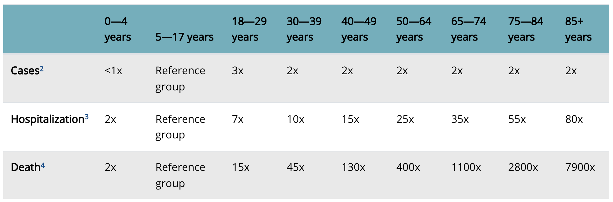
Our first model will be based on the statistics collected by the Centers for Disease Control and Prevention (CDC). That’s right; sometimes, we don’t need raw data to build a predictive model. We’ll start by turning a table with mortality statistics into a predictive model.
Note, that the risk for the reference group is not included in Figure 1. To calculate the mortality predictions we use here the baseline relative risk determined on Polish data at the beginning of Covid pandemic, which is 0.003% for the reference group. Currently, it is far much smaller as a large fraction of the population is already immunized.
Python snippets
We follow the common convention in Python that a model is an object that has predict function, which transforms the \(n\times p\) input matrix with \(p\) variables for \(n\) observations into a vector of \(n\) predictions. Below, we define a class cdc_risk that calculates the odds of Covid related death based on statistics from the CDC website.
Different machine-learning libraries may create models represented by objects with different structures. To automate the processing of models we need a uniform standardized interface. Here, we use the abstraction implemented in the dalex package Baniecki et al. (2021).
Baniecki, Hubert, Wojciech Kretowicz, Piotr Piatyszek, Jakub Wisniewski, and Przemyslaw Biecek. 2021. “Dalex: Responsible Machine Learning with Interactive Explainability and Fairness in Python.” Journal of Machine Learning Research 22 (214): 1–7. http://jmlr.org/papers/v22/20-1473.html.
The Explainer constructor creates an Explainer object, i.e. a wrapper for a predictive model that has API consistent with other functions from dalex package. The first argument is a model. It can be an object of any class but it is assumed that the object contains the predict function as in our example. The label specifies a unique name that appears in the plots while other arguments are introduced in the next sections.
import dalex as dx

explainer_cdc = dx.Explainer(model_cdc, label="CDC")
explainer_cdc.predict(steve)
## array([0.00045])
Using the Explainer may seem like an unnecessary complication at the moment, but on the following pages, we show how it simplifies our work.
R snippets
We follow the common convention in R that a predictive model is a function that transforms the \(n\times p\) data frame with \(p\) variables for \(n\) observations into a vector of \(n\) predictions. For further examples, below, we define a function that calculates the odds of Covid related death based on statistics from the CDC website for different age groups.
cdc_risk <- function(x, base_risk = 0.00003) {
  rratio <- rep(7900, nrow(x))
  rratio[which(x$Age < 84.5)] <- 2800
  rratio[which(x$Age < 74.5)] <- 1100
  rratio[which(x$Age < 64.5)] <- 400
  rratio[which(x$Age < 49.5)] <- 130
  rratio[which(x$Age < 39.5)] <- 45
  rratio[which(x$Age < 29.5)] <- 15
  rratio[which(x$Age < 17.5)] <- 1
  rratio[which(x$Age < 4.5)]  <- 2
  rratio * base_risk
}

steve <- data.frame(Age = 25, Diabetes = "Yes")
cdc_risk(steve)
## [1] 0.00045
Predictive models implemented in different libraries have different structures. To automate our work we need a standardized interface, so we use the abstraction implemented in the DALEX package Biecek (2018).
Biecek, Przemyslaw. 2018. “DALEX: Explainers for Complex Predictive Models in R.” Journal of Machine Learning Research 19 (84): 1–5. https://jmlr.org/papers/v19/18-416.html.
The explain function from this package creates an explainer, i.e. a wrapper for the model that will allow you to work uniformly with objects of very different structures. The first argument is a model. It can be an object of any class, e.g. a function (functions as objects in R). The second argument is a function that calculates the vector of predictions. DALEX package can often guess which function is needed for a specific model, but in this book, we show it explicitly in order to emphasize how the wrapper works. The type argument specifies the model type and the label specifies a unique name that appears in the plots.
library("DALEX")
model_cdc <- DALEX::explain(cdc_risk,
               predict_function = function(m, x) m(x),
               type  = "classification",
               label = "CDC")
predict(model_cdc, steve)
## [1] 0.00045
Using the explain function may seem like an unnecessary complication at the moment, but on the following pages, we show how it simplifies the work.