Step 9. Ceteris Paribus

Once we know which variables most influenced the model’s prediction for a particular instance, the next question we want to answer is how and how much the variables affected this individual prediction. This leads to an analysis of the model’s response profiles as a~function of individual variables. We have already performed such an analysis at the global level using Partial Dependence profiles. But for complex models, the local behaviour may diverge from the global, especially if we analyze observations from low-density regions. The tool we will use for local profile analysis is Ceteris Paribus curves.

Ceteris Paribus (CP) is a Latin phrase for “other things being equal”. It is also a very useful technique for an analysis of model behaviour for a single observation. CP profiles, sometimes called Individual Conditional Expectations (ICE), show how the model response would change for a selected observation if a value for one variable was changed while leaving the other variables unchanged.

More formally, for a model \(f(x)\), variable \(i\) and observation \(x^*\) the CP profile is a function

\[ CP(t,i,x^*) = f(x^*_1, \cdots, x^*_{i-1}, t, x^*_{i+1}, \cdots, x^*_p). \]

Note that if variable \(i\) is correlated with other variables, changing its value independently of other variables can lead to off-manifold observations, so CP profiles should be analyzed with caution.

While local variable attribution is a convenient technique for answering the question of which variables affect the prediction, the local profile analysis is a good technique for answering the question of how the model response depends on a particular variable. Or answering the question of what if…

Python snippets

The predict_profiles() function calculates Ceteris Paribus profiles for a selected model and selected observations. By default, it calculates profiles for all variables, but one can limit this list with the argument variables. The calculated profiles can be drawn with the plot function.

cp_steve = explainer_rfc_tuned.predict_profile(Steve)

Here we plot CP for Age.

cp_steve.plot(variables="Age", show=False)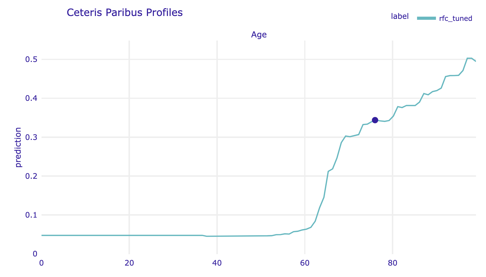

Figure 1: CP profiles for Steve. The dot shows the observation under analysis. CP profile shows how the model predictions change for changes in the selected variable. On the left is the CP profile for the continuous variable `Age`, on the right for the categorical variable `Cardiovascular.Diseases`. For categorical variables, one can specify how the CP profiles should be drawn by setting the `categorical_type` argument.

As with other explanations in the dalex library, multiple models can be plotted on a single graph.

cp_cdc = explainer_cdc.predict_profile(Steve)
cp_dtc = explainer_dtc.predict_profile(Steve)
cp_rfc = explainer_rfc.predict_profile(Steve)

cp_cdc.plot([cp_rfc, cp_dtc, cp_steve], 
        variables="Age", show=False)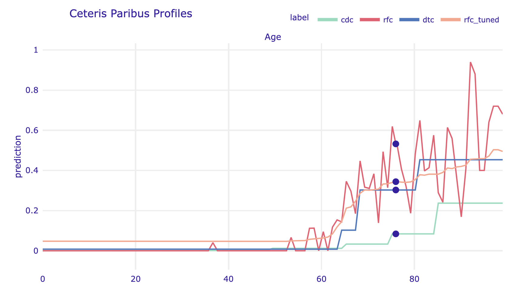

Figure 2: CP profiles for Steve, colors code four considered models.

R snippets

cp_ranger <- predict_profile(model_ranger, Steve)
cp_ranger
#  Top profiles    : 
#       Gender   Age Cardiovascular.Diseases Diabetes
# 1     Female 76.00                     Yes       No
# 1.1     Male 76.00                     Yes       No
# 11      Male  0.00                     Yes       No
# 1.110   Male  0.99                     Yes       No

The calculated profiles can be drawn with the generic plot function. As with other explanations in the DALEX library, multiple models can be plotted on a single graph. Although for technical reasons quantitative and qualitative variables cannot be shown in a single chart. So if you want to show the importance of quality variables, you need to plot them separately.

Figure 3 shows an example of a CP profile for continuous variable Age and categorical variable Cardiovascular.Diseases. For categorical variables, one can specify how the CP profiles should be drawn by setting the categorical_type argument.

plot(cp_ranger, variables = "Age")
plot(cp_ranger, variables = "Cardiovascular.Diseases", 
        categorical_type = "lines")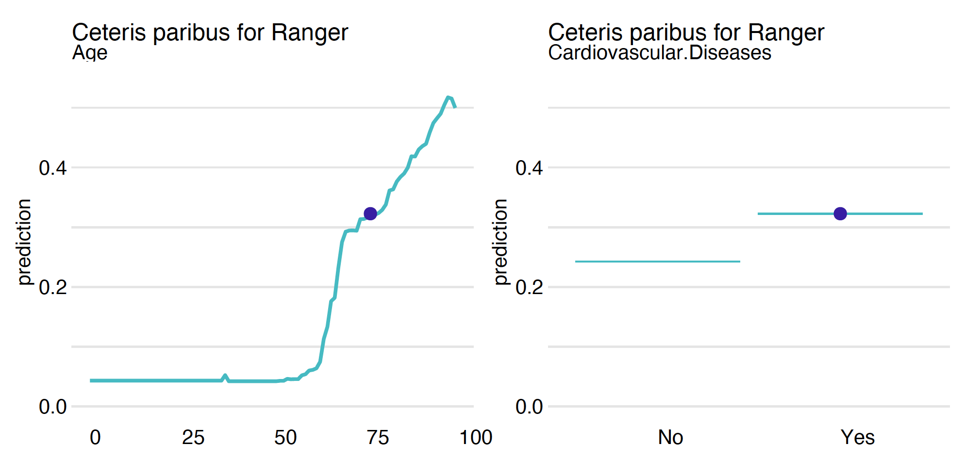

Figure 3: CP for Steve calculated for the random forest model. The dot shows the observation under analysis. CP profile shows how the model predictions change for changes in the selected variable. On the left is the CP profile for the continuous variable `Age`, on the right for the categorical variable `Cardiovascular.Diseases`.

The plot function can combine multiple models, making it easier to see similarities and differences. In our case, we work with models based on step functions (handcrafted rules, trees, random forests), and even within such similar models, we can see differences in behaviour. These differences will be even greater if we include models with smooth responses, such as linear models, Support Vector Machines or neural network models.

cp_cdc <- predict_profile(model_cdc, Steve)
cp_tree <- predict_profile(model_tree, Steve)
cp_tune <- predict_profile(model_tuned, Steve)

plot(cp_cdc, cp_tree, cp_ranger, cp_tune, variables = "Age")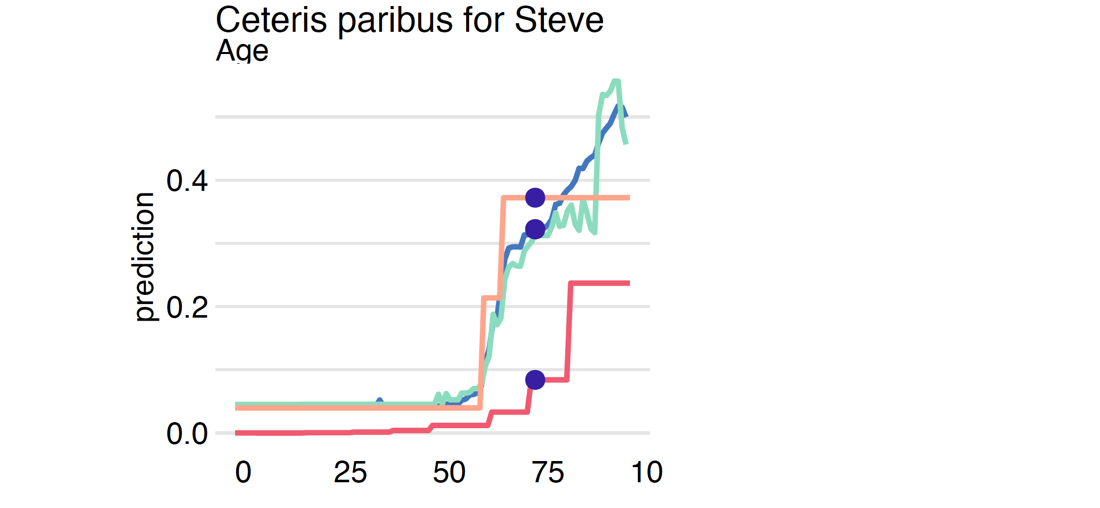

Figure 4: CP profiles for Steve, colors code four considered models.

Note that in the example analyzed, the largest differences between the analyzed models are in the group of the oldest patients. In the CDC model, a significant jump in mortality was observed for the group of people over 80 years old, while in the models trained on the data, mortality increases very rapidly from age 60 and quickly reaches very high values.

The size of the oscillation can be measured in many ways, by default, it is an area between the CP profile and a horizontal line at the level of the model prediction.

Variable importance through oscillations

CP profiles have many applications, both in analyzing the stability of a model and in determining which variables are important.

When we examine the stability of a model, we may be concerned about large local variability in the CP profile, lack of monotonicity, and isolated narrow peaks. It turns out that such artefacts can often be seen on profiles for random forest models.

When assessing the importance of variables, the following intuition accompanies the reasoning. The more the CP profiles fluctuate, the more influential the variable is. A measure of importance based on this intuition is implemented in the predict_parts function under option type = "oscillations". The size of the oscillation can be measured in many ways, by default, it is an area between the CP profile and a horizontal line at the level of the model prediction.

predict_parts(model_ranger, Steve, type = "oscillations")
#                   _vname_ _ids_ oscillations
# 2                     Age     1   0.22872998
# 6         Kidney.Diseases     1   0.16371903
# 7                  Cancer     1   0.09641507
# 4                Diabetes     1   0.05052652
# 3 Cardiovascular.Diseases     1   0.03984208
# 1                  Gender     1   0.03308303
# 5   Neurological.Diseases     1   0.03164090

Is this the end?

PD, ALE, CP profiles, SHAP, Break down or permutational importance of variables have revealed a lot about the behaviour of considered models. However, they do not completely explore the possible scenarios for model analysis. One can dig deeper into the analysis of groups of variables or analysis of residuals.

Based on the first iteration of the modelling process, we gain new knowledge of which variables are important (primarily age) what is the relationship between them and mortality (monotonic but not linear, more exponential or polynomial), which other variables are important (such as cardiovascular diseases). Equipped with this knowledge, we now can develop new models. But due to the limited volume of the book, we leave it to readers’ own experiments.